The Tracking module
 In the previous module, we saw how features can be automatically extracted from images using FAST. Bespoke features can also be externally defined using alternative techniques. In all cases however, features are numerical, instantaneous and assignable (to a single object at a given timepoint). Examples include object shape, position or colour.
How information from all these different features can be optimally combined to maximise tracking fidelity is not immediately obvious. As a toy example to explore this problem, we might imagine filling an opaque box with uniquely coloured marbles, closing it and giving it a shake. Upon opening the box, how could we match the ones we see inside with the ones we put in the box? Because we were unable to track the positions of the marbles as we shook them, positional information would be useless. However, an accurate assignment could still be made based on their unique colour. In this case therefore, we would wish to weight the colour information much more strongly than the positional information.
At the core of FAST's tracking algorithm are methods to automatically perform this type of weighting, allowing many features to be easily combined. This page will focus on the practical aspects of using the FAST tracking GUI; for more detailed information about the algorithm used, please refer to this page.
To begin the tracking GUI, click the 'Tracking' button on the home panel. You should now see the following GUI appear:
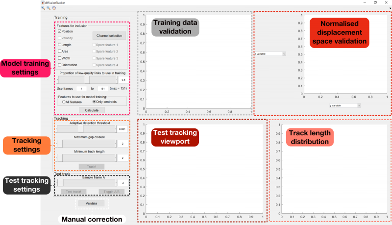
Model training
In the model training stage of the algorithm, a set of low-fidelity links are made between each pair of frames in the dataset. Statistical properties are then extracted from these links, and are used to perform high-quality tracking in the next stage of the algorithm.
Feature choice
Crucial to the overall performance of the tracking algorithm are the features that are included in the analysis. Good features possess two key properties: firstly, they are robust, remaining stable over large periods of time. It is easier, for example, to track static objects than ones that are rapidly moving. Secondly they are diverse, with substantial variation between different members of the population of objects - it is far easier to track a set of objects on the basis of colour if they span the whole spectrum, rather than just being slightly different shades of green.
Some features can also be useful for telling the algorithm when something has gone wrong. For example, an object may mis-segment, maintaining approximately the same position but substantially reducing its apparent length. As long as cell length is included as a feature (and assuming it is fairly robust), the algorithm will be able to automatically detect this mis-segmentation and throw it out.
The checkboxes in the Features for inclusion panel allow you to choose the features within your dataset that fulfil the above criteria.
Position is almost always the most powerful feature available, and is always selected. Externally defined features can be chosen as Spare feature 1, Spare feature 2 etc. if they have been prepared as described in the relevant section.
Training link inclusion proportion choice
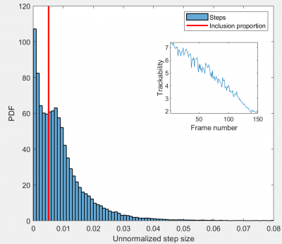
Once you have chosen the features you wish to include, click Calculate!. Once this has finished processing, a histogram will appear in the top-left hand axes. This can be used to select the first of the user-defined parameters, denoted as Proportion of low-quality links to use in training. Changing the value of this parameter with either the slider or the edit box will alter the position of the vertical red line plotted on top of the histogram.
This histogram indicates the initial distribution of frame-frame link distances, before any feature reweighting has been performed. Typically, it contains two peaks, one towards the left containing accurate links, and one further to the right containing the inaccurate links. If this is the case, it is usually best to select the Proportion of training links to use parameter to split these populations in two. An example is shown below:
If there are more than two peaks, choose a value that splits the left-most peak from the others.
If you see only a single peak, try changing the Features to use for model training radio button selection to All features. This will switch the training portion of the algorithm from using only object position to assign the initial set of links to using the entire set of selected features. If object position is of a similar reliability to the other features included in the model training, adding them into the training stage can improve the accuracy of initial link assignment. If this still results in a single peak, revert back to Only centroids and choose a Proportion of training links to use that sits just to the right of the peak.
Once you have finalised your selection, click Calculate! again to generate your final statistical model of the dataset.
The trackability plot
Above and to the right of the main histogram, a second pair of axes indicate the time evolution of the trackability of the dataset. This provides a heuristic view of the ease of tracking the given dataset over time. In the example above, the trackability decreases monotonically over the course of the dataset, due to a) a gradual increase in object number, and b) a gradual increase in object motility. The boxes $t_1$ and $t_2$ in Use frames $t_1$ to $t_2$ (max = $t_{max}$ ) can be used to limit the timepoints included in the analysis to those above a certain trackability. If adjusted, the Calculate! button will again need to be pressed to retrain the model on the more limited dataset.
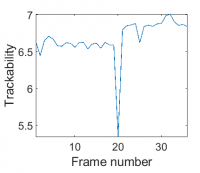
Trackability can also be used to automatically detect problems in the original datasets. In the example below, the global intensity of the segmented phase-contrast image increased suddenly at frame 20, causing the area and length of the segmented objects to instantaneously increase by a small amount. This effect can be observed as a sudden drop in the trackability of the dataset at the offending timepoint.
Tracking
Once the tracking model has been trained, it can be applied to the whole dataset. Thanks to its ability to automatically weight all included features appropriately, only one parameter needs to be adjusted to change the stringency of tracking: the adaptive detection threshold.
Adaptive detection threshold choice
The most useful tool for determining what value this parameter should take is the Test track box. This applies the given value to a single frame of your dataset and plots the result, allowing you to check how the stringency of the algorithm should be adjusted.
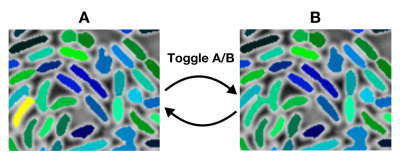
To use it, simply click the Test Track! button. Once it has finished processing, an image should now appear within the bottom left-hand axes. This contains the first frame (A) of your test track. To see the second (B), click the Toggle A/B button. Clicking this button again will take you back to frame A, as indicated below:
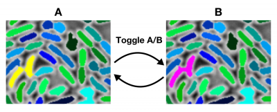
Objects are overlaid with masks of one of three types, indicated by colour:
- Green and blue objects have been assigned links between the two frames. The colour of linked objects remains constant between the two frames.
- Yellow objects are objects in frame A that have not had a link assigned to an object in frame B, as their associated score was below the currently selected linking threshold.
- Purple objects are objects in frame B that have not had a link assigned from an object in frame A.
In the case above, most objects have been assigned links and are correspondingly coloured green or blue. The exception to this is the pair of objects in the bottom left-hand corner of the image. They are initially segmented correctly in frame A, but become fused in frame B. Because of this mis-segmentation, the tracking algorithm has correctly rejected any link to or from these objects.
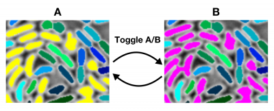
Increasing the adaptive threshold to too high a value will allow false links to be accepted:
While reducing it to too low a value will cause true links to be rejected:
If you want to check multiple timepoints in your dataset (possibly because of large variations in trackability over time), you can use the Sample frame A slider and edit box to choose which frame will form frame A of the test track output.
The normalised displacement space viewport
After you have performed test tracking, you can view the normalised displacement space for the selected frame in the top right-hand viewport. By selecting different options from the dropdown menu, different pairs of features from the multidimensional feature space can be compared. This window assists in two tasks.
Firstly, it can be used to verify that each feature is properly normalised. If they have been properly normalised, the displayed scatterplot should be isotropic (radially symmetric) and centred on the origin. Below are examples of well-normalised (left) and poorly normalised (right) features:
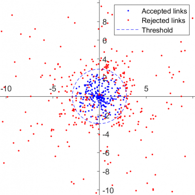
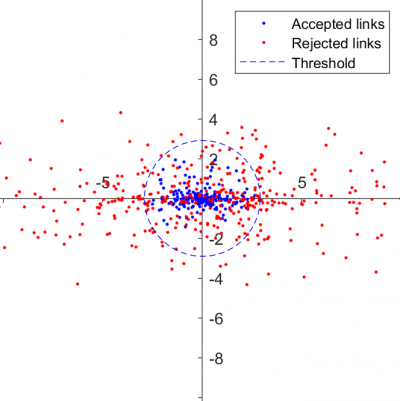
In the second case, the 'squashed' shape of the scatterplot indicates that the feature used for the y-axis has been poorly normalised. This can be confirmed by choosing other features to display on the x-axis - if the y-axis feature has not been properly normalised, each resulting scatterplot will appear non-isotropic.
- Choosing the only centroids option in the Features to use for model training panel.
- Increasing the proportion of low-quality links used in model training.
- Unchecking the box corresponding to the offending feature in the Features for inclusion panel.
Secondly, it can be used as a second means of refining the adaptive detection threshold. The current threshold is shown as a blue dashed circle, with accepted test links shown in blue and rejected test links in red. As the threshold is manually changed, the plotted circle will vary accordingly, allowing you to choose a value that best separates 'true' links (inside the circle) from 'false' links (outside the circle).
Gap-bridging
Mistakes that occur at one timepoint may be fixed at later timepoints. In the case of the yellow/purple cells above, perhaps the mis-segmented purple cell is correctly broken into two objects again at subsequent timepoints. To account for these cases, FAST incorporates a gap-bridging component that allows these short-lived mistakes to be skipped over without breaking the track. To use it, simply set Maximum gap closure to a value greater than 1 (the default is 2). This parameter indicates the maximum number of timepoints the gap-bridging algorithm is allowed to cross in its search for an object to link a broken trajectory to.
Once you are happy with your parameter selections, click the Track! button to begin tracking the entire dataset.
Post-processing
After tracking has finished, FAST allows the resulting tracks to be edited in two ways:
Track length filtering
Various processes can generate short tracks that are not useful for analysis. Mis-segmentations can result in 'objects' that appear for only a single frame, objects can move in and out of the field of view over a very short period of time, or highly stringent tracking can break tracks into many short pieces. The extent of these effects can be seen by looking at the track length distribution, plotted in the lower right panel once tracking has finished:
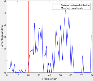
This shows the percentage of detected objects that are assigned to tracks of each length. For example, a value of 4 at track length 15 indicates that 4% of objects were assigned to tracks of length 15. Also shown is a red vertical line, indicating the track length threshold. To remove short tracks, adjust the Minimum track length slider. The red vertical line will move accordingly, allowing you to see how much of the distribution (everything to the left of the line) has been removed.
Track data is automatically filtered and saved as the Minimum track length parameter is changed.
Manual correction
FAST also supports manual correction of tracks. To begin the track correction GUI, click the Validate button in the lower left hand corner of the tracking GUI. Full details on how to use this GUI can be found here.
Outputs
Once you have completed tracking, a new file named 'Tracks.mat' will be saved in your root directory. Several data structures are saved within this file:
- toMappings and rawToMappings: Structures for mapping from the 'slice' representation of trackableData to the 'track' representation of procTracks. rawFromMappings contains the mappings generated by the tracking algorithm, fromMappings contains the mappings once manual correction has been applied.
- fromMappings and rawFromMappings: Structures for mapping from the 'track' representation back to the 'slice' representation. These allow features that can only be calculated in the track representation (such as object speed) to be converted back to the slice representation.
The 'slice' and 'track' representations of the dataset are stored in trackableData and procTracks, respectively. In general, the following statements should be true:
  procTracks(a).x(b) == trackableData.Centroid{toMappings{a}(b,1)}(toMappings{a}(b,2),1)
  trackableData.Centroid{c}(d,1) == procTracks(fromMappings{c}(d,1)).x(fromMappings{c}(d,2))
for all a, b, c and d. These expressions generalise for all other fields than trackableData.Centroid and procTracks.x.
- procTracks: The full set of track data.
- linkStats: The statistics associated with each of the features, calculated during the model training stage.
- trackTimes: The times at which each track was sampled.
- trackableData: Raw feature data. Identical to the main output of the feature extraction module.
- trackSettings: The settings selected in the feature tracking GUI.
Of these, the most important and complex is procTracks. This structure contains the tracked feature data for all objects in your dataset. It is organised as shown below:

Unless you have added additional features prior to object tracking, procTracks will initially contain the following fields:
- x and y: The instantaneous coordinates of the object over time. Each is a $t \times 1$ vector.
- theta and vmag: The instantaneous direction of motion (in degrees) and speed of the object. Each is a $(t-1) \times 1$ vector.
- times: The timepoints the object's position was sampled at. As gaps in tracks can be bridged, this list of timepoints is not necessarily contiguous. A $t \times 1$ vector.
- length: Total length (in timepoints) of the track.
- start and end: Start and end timepoints of the track.
- age: The age of the object relative to the start of the track at each timepoint. Equivalent to times - start.
- interpolated: $(t-1) \times 1$ logical vector indicating whether there was a gap in the track at this timepoint. If so, values in all other fields for this timepoint have been linearly interpolated from surrounding values.
Depending on the options selected in the feature extraction module, additional fields may also be available:
- majorLen and minorLen: The length and width of the object at each timepoint. Each is a $t \times 1$ vector.
- area: The (projected) area of the object at each timepoint. A $t \times 1$ vector.
- phi: The orientation of the object at each timepoint in degrees. A $t \times 1$ vector.
- channel_n_mean: The average intensity of the object at each time point in each analysed channel. Each is a $t \times 1$ vector.
- channel_n_std: The standard deviation of the object's intensity in each analysed channel at each timepoint. Each is a $t \times 1$ vector.
Additional fields, such as population and event labels, can be added as described in the advanced usage section.